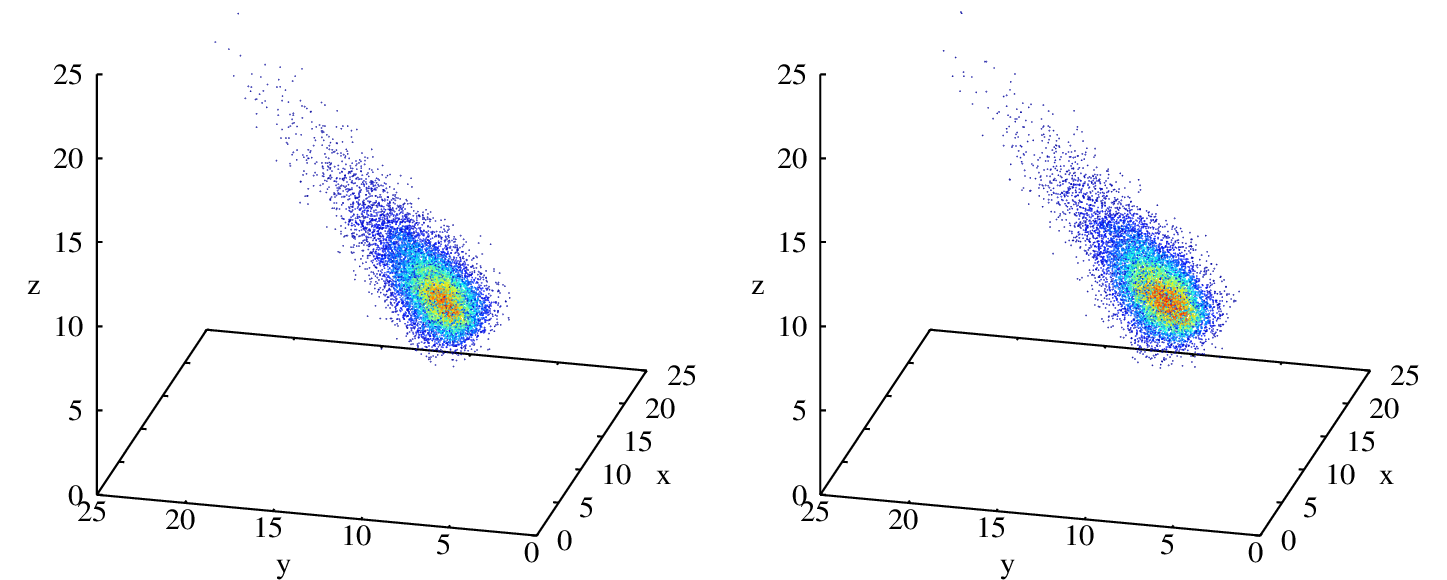
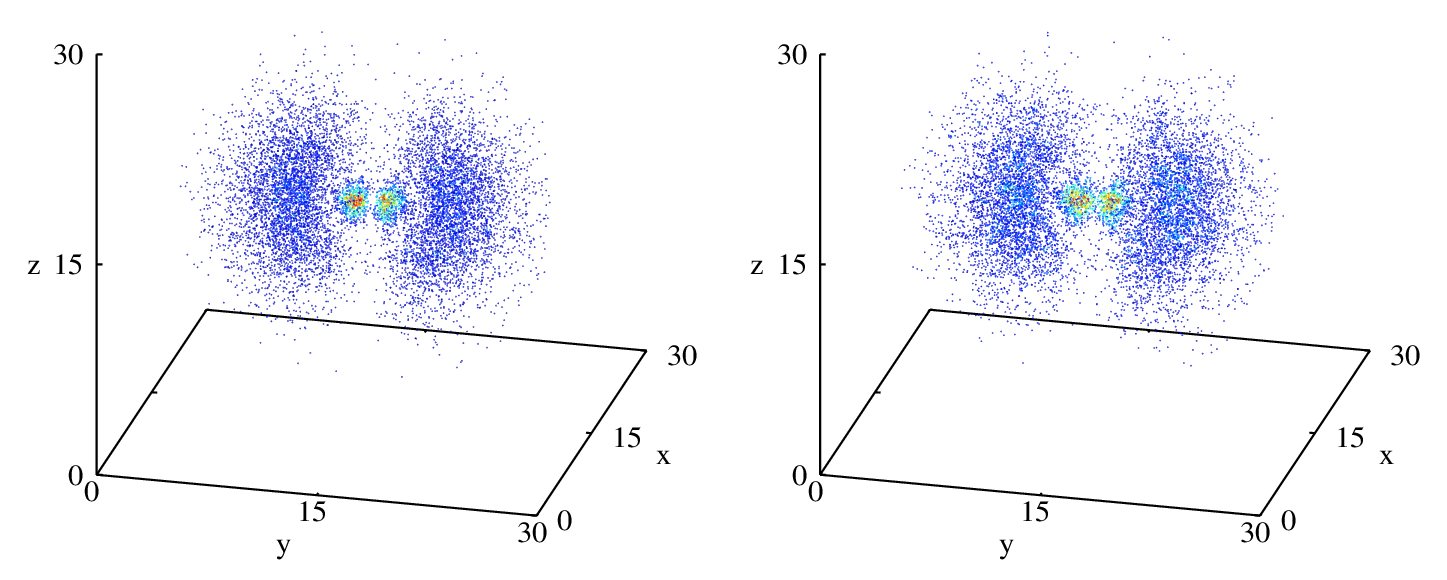
mveqf
Multivariate Empirical Quantile Function (grid-based)
- Let \({\mathbb{R}}\) denote the set of all real numbers.
- Let \(X\) be a random vector on a probability space \((\Omega ,{\mathcal {F}},P)\) with distribution function \(F_{X}:{\mathbb{R}} \rightarrow [0,1]\), where \({F}_X(x) = \mathrm{P}(X \leq x)\).
- The quantile transform \(F_{X}^{-1}:[0,1] \rightarrow {\mathbb{R}}\) for \(F_{X}\) is \(F_{X}^{-1}(p) = \mathrm{inf}\{ x \in {\mathbb{R}} : P(X \leq x) \geq p \}\).
-
The empirical distribution function is defined as \(\hat {\mathrm{F} }_X (u) = \frac{1}{n} \sum\limits_{\substack{i=1}}^n \mathbf{1} (\mathbf {x}_{[i]} \leq u)\), where \(\mathbf{1}\) is the indicator function.
- Using the definition of the multivariate empirical distribution function
where \(d\) – dimension, \(n\) – sample size, it is possible to define a multivariate quantile function \([0,1]^{d} \rightarrow {\mathbb{R}}^{d}\).
- Let \(F\) be a \(d\)-dimensional distribution function, \(X_{1}, \ldots, X_{n}\) be the sample. Then for given vector \(z \in [0,1]^{n}\) using univariate quantile transform the multivariate quantile function \(Y = \tau_{F}^{-1}(z)\) is defined recursively as

